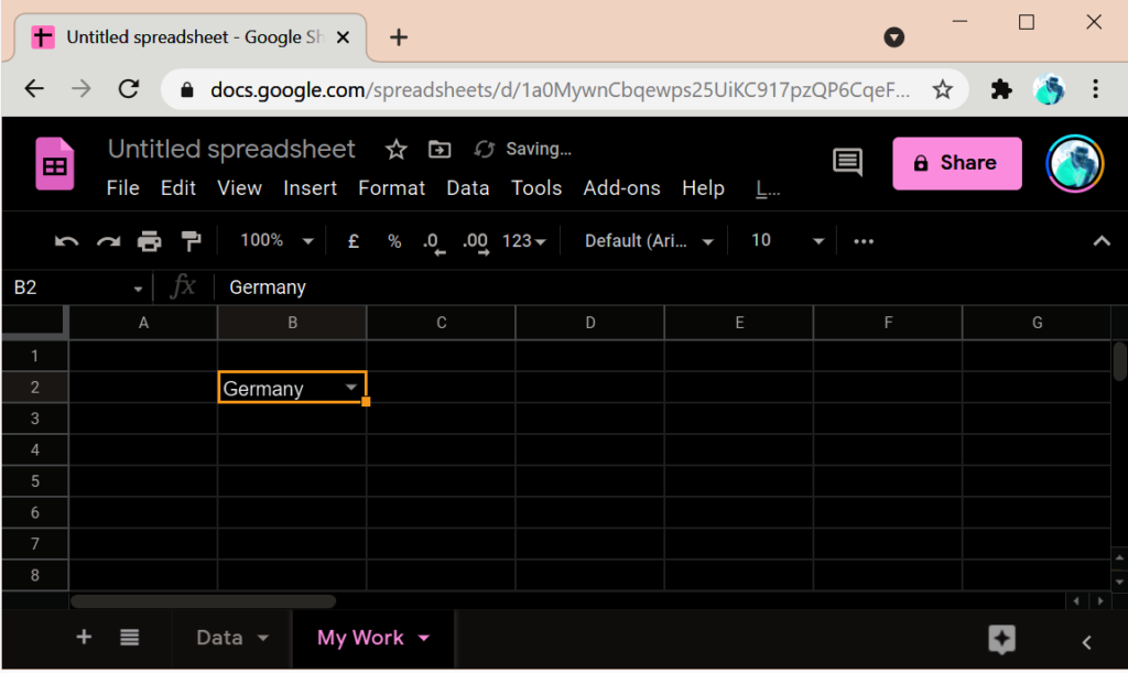
Excel of Microsoft Office has a very powerful feature of creating drop downs.
Benefits:
- Validation of data, as wrong data can’t be entered
- Faster data entry
In this blog we will follow step-by-step procedure to do create the dropdown validation.
1. In a new sheet enter the data values (can be added & deleted later) for the dropdown.
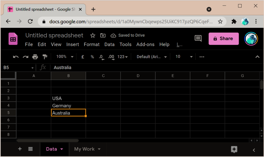
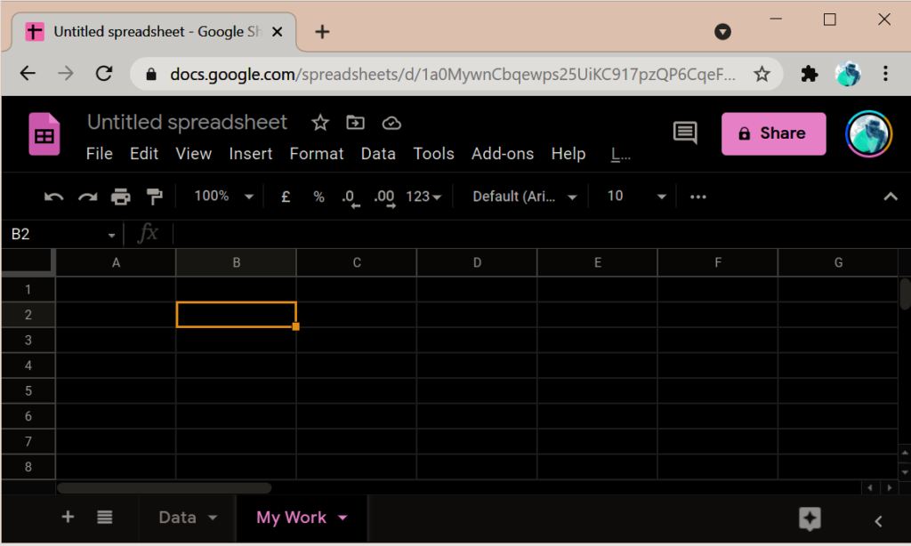
2. Create a new sheet and select cell(s) where the dropdown will appear. Once dropdown is set for a cell, you can copy paste the dropdown in other cells.
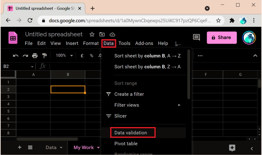
3. From Menu Bar select “Data” => “Data Validation”
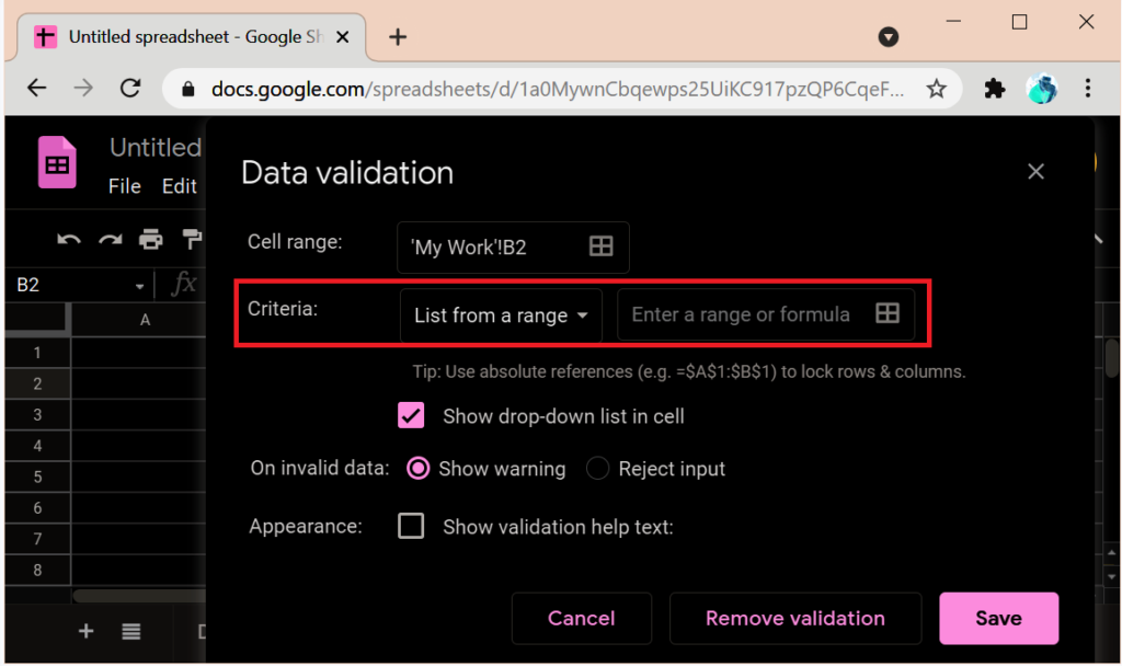
4. This will open “Data Validation” window. From “Criteria” dropdown select “List from a range” and click “Enter a range or formula”. This will open a floating window to accept the data value range.
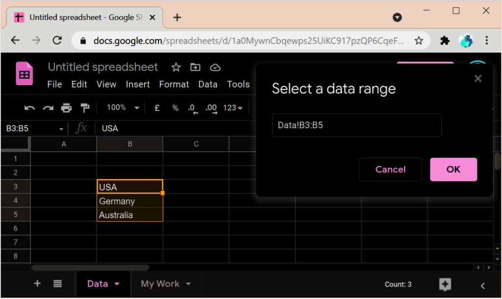
5. Select your data range (selecting entire column will make it more versatile; as you can add new data to get in dropdown without changing the formula). The cell(s) formula is automatically taken by the “Select a data range” text box.
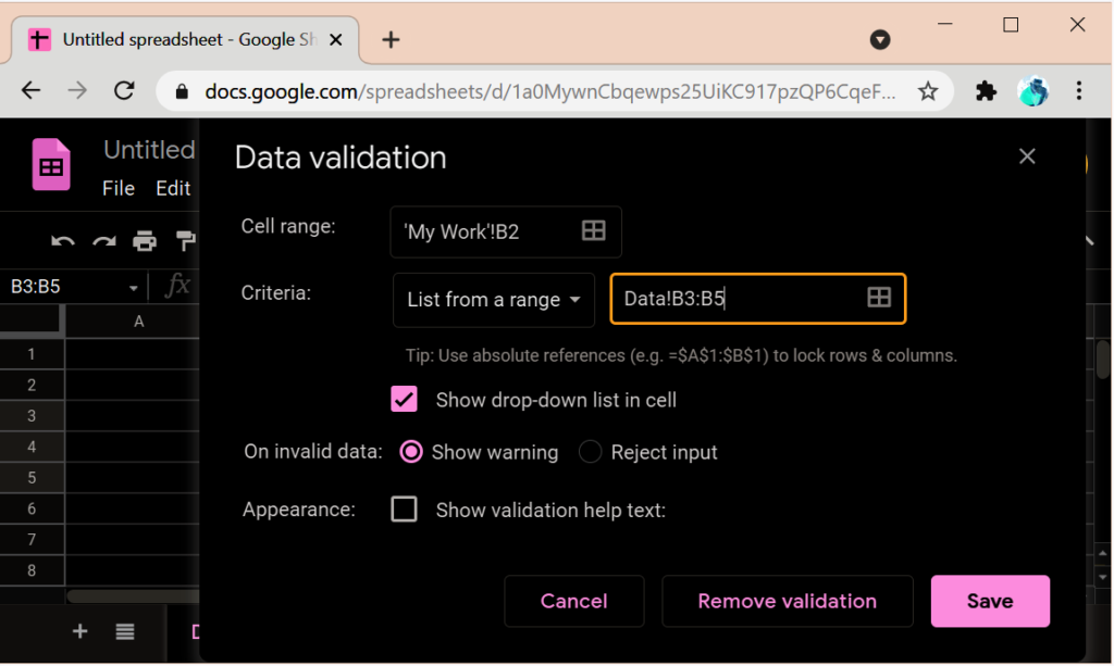
6. Hit Enter to chose the data range and then “Save” to confirm.
7. Clicking the dropdown shows the data values.
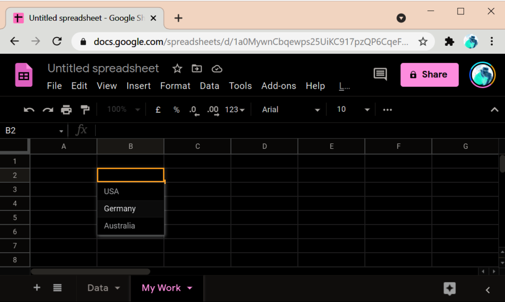
8. Select your value and you are all done.
